


Next: Electromagnetic Waves
Up: From the Maxwell Equations
Previous: From the Maxwell Equations
Contents
Electromagnetic waves are the carrier of
all target relevant information between a given radar and a distant target observed
by that radar.
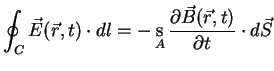
Michael Faraday (1791-1867) discovered, that a time varying magnetic flux
 through a closed conducting loop induces an electromagnetic field around that loop.
 |
(A.1) |
where
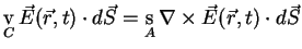
 is the electric field intensity vector, C a closed path around
and
A the open area bounded by C. This rule is known as Faraday's Induction Law,
stating that a time varying magnetic field is always connected
to an electric field.
is the electric field intensity vector, C a closed path around
and
A the open area bounded by C. This rule is known as Faraday's Induction Law,
stating that a time varying magnetic field is always connected
to an electric field.
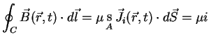
The second important equation, known as the Ampère 's Circuital Law, was found
by André Marie Ampère (1775-1836). This equation relates a line integral of
tangent to a closed curve C, with the total current i passing within the confines of C.
 |
(A.2) |
where
 is the induced current density and
  is the relative
permeability tensor
for the given media. Even though the equation above is valid for many applications
it does not yield the whole truth. Moving charges are not the only source of
a magnetic field, e.g. the for the case of charging a capacitor a B-field can
be measured between the plates, even though no current traverses the capacitor.
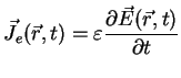
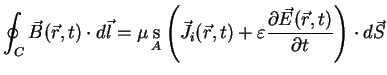
James Clerk Maxwell (1831-1879), therefore, predicted the existence of a another type of current-flow
mechanism, called displacement current density
is the relative
permeability tensor
for the given media. Even though the equation above is valid for many applications
it does not yield the whole truth. Moving charges are not the only source of
a magnetic field, e.g. the for the case of charging a capacitor a B-field can
be measured between the plates, even though no current traverses the capacitor.
James Clerk Maxwell (1831-1879), therefore, predicted the existence of a another type of current-flow
mechanism, called displacement current density

 |
(A.3) |
where
 is the dielectric constant leading to a new and complete formulation of (A.2)
 |
(A.4) |
meaning that a time varying E-field is always accompanied by an magnetic B-field,
even when
 .
The remaining two Maxwell equations refer to Karl Friedrich Gauss (1777-1855).
The first one denotes the relation between the electric field
through
a closed surface A and the charges contained in the volume V surrounded
by A.
.
The remaining two Maxwell equations refer to Karl Friedrich Gauss (1777-1855).
The first one denotes the relation between the electric field
through
a closed surface A and the charges contained in the volume V surrounded
by A.
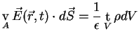 |
(A.5) |
where  is the electric charge density and
  is a vector perpendicular to
A pointing outwards.
This equation is sometimes referred as the coulomb law.
is a vector perpendicular to
A pointing outwards.
This equation is sometimes referred as the coulomb law.
Due to the fact, that no magnetic monopoles are known to exist, the equivalent of the
equation above for the magnetic flux  is given by
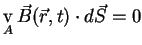 |
(A.6) |
The set of the four integral equations are know as
the Maxwell Equations and describe the behavior and relation of electromagnetic
fields. These equations can be also written in differential formulation which is
better suited to derive the wave aspects of the electromagnetic field. In order to change
from the integral to the differential formulation Gausses theorem
(1813)
 |
(A.7) |
and Stokes' theorem (1854)
 |
(A.8) |
are applied, where  denotes a vector field.
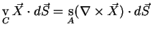
By applying Stokes' theorem to the electric field we get
denotes a vector field.
By applying Stokes' theorem to the electric field we get
 |
(A.9) |
Comparing this result with (A.1) we find
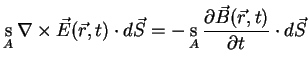 |
(A.10) |
This must be true for all surfaces A confined by C, which is only the case if the arguments under the
integrals are equal, hence
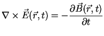 |
(A.11) |
In exactly the same way (A.4) is translated into
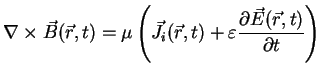 |
(A.12) |
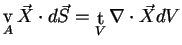
Gausses theorem applied to the electric field yields
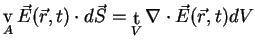 |
(A.13) |
and with (A.5) we get
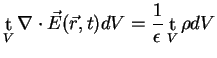 |
(A.14) |
which in the differential form yields
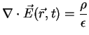 |
(A.15) |
Analogous application of Gausses theorem to (A.5) leads to
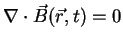 |
(A.16) |
With these equations, which are valid for all times t and all points
in space  , the behavior of electromagnetic fields is unambiguously
described by the real quantities
,
,
, the behavior of electromagnetic fields is unambiguously
described by the real quantities
,
,
 and
and
 .
.
Next: Electromagnetic Waves
Up: From the Maxwell Equations
Previous: From the Maxwell Equations
Contents