Next: Processing of SAR-data Up: processing Previous: Short overview on SAR
Main level: Epsilon Nought - Radar Remote Sensing

Subsections

Synthetic Apertur Radar

Principles of radar imaging

The objective of radar imaging is to generate a two-dimensional reflectivity map of an examined scene in the microwave region of the electromagnetic spectrum. Radar systems are commonly based on the measurement of signal time delays (RADAR = Radio Detection And Ranging) [55]. A normal monostatic imaging radar system consists of a microwave transmitter and receiver, operated on a moving platform like an air-plane or satellite. In the simplest case the antenna is oriented parallel to the flight direction, i.e. it is looking sidewards to the ground (see Fig. 2.1). The look direction of the antenna is normally called ` range' or ` slant-range'. The transmitter emits fast consecutively short radar pulses to the ground. These pulses are reflected from a scatterer on the ground and after a certain time delay $\Delta t$ they reach again the receiver. This time delay is a function of the distance between the sensor and the scatterer

$\begin{displaymath}\Delta t = \frac{2r}{c} \quad,\end{displaymath}$

(1)

where denotes the speed of light. Different scatterers can be resolved because their echos show different time delays. Thus, the achievable resolution $\delta_{sr}$ in slant-range is dependent on the transmitted pulse length $\tau$ , or alternatively, on the bandwidth of the pulse

$\begin{displaymath}\delta_{sr} = \frac{c\tau}{2} = \frac{c}{2W}\quad.\end{displaymath}$

(2)

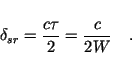
Obviously, the range resolution is independent of the distance between the scatterer and the sensor. To achieve high resolution in range, very short pulse durations are necessary. The resulting energy densities are often difficult to handle in practice. Therefore, in modern radars, normally a high bandwidth is reached by transmitting a longer pulse with a linear frequency modulation (chirp) instead. The energy of this pulse is distributed over a longer duration, but it can be compressed again after receiving it by a matched filtering operation [56]. For example, a bandwidth of 100MHz corresponds to a resolution of 1.5m.

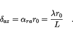
In the along track or azimuth direction, the resolution of a simple side-looking radar corresponds to the size of the antenna footprint on the ground. The angular resolution $\alpha_{ra}$ of an antenna of length in the azimuth direction is limited due to diffraction effects on its aperture. For a wavelength of $\lambda$ it is given by

$\begin{displaymath}\alpha_{ra} = \frac{\lambda}{L} \quad.\end{displaymath}$

(3)

The spatial resolution in azimuth at a given range then results as

$\begin{displaymath}\delta_{az} = \alpha_{ra} r_0 = \frac{\lambda r_0}{L} \quad.\end{displaymath}$

(4)

Apparently, the resolution in azimuth decreases with increasing flight heights and the corresponding longer distances to the object. High resolution in azimuth requires large antennas and short object distances. For example, spaceborne systems with an orbital height of 800km and an antenna aperture of 15m would show only a resolution of approximately 3km.

$\includegraphics [width=14cm]{bas_sargeo.epsi}$

Figure 2.1: Left: SLAR/SAR imaging geometry in strip-map mode. Right: geometric representation of the maximum possible synthetic aperture length $L_{sa}$

Resolution of a synthetic aperture radar

A Synthetic Aperture Radar (SAR) overcomes these problems and is designed to achieve high resolutions with small antennas over long distances [57]. A SAR system takes advantage of the fact that the response of a scatterer on the ground is contained in more than a single radar echo, and shows a typical phase history over the illumination time. An appropriate coherent combination of several pulses leads to the formation of a synthetically enlarged antenna - the so-called ` synthetic aperture'. This formation is very similar to the control of an antenna array, with the difference that only one antenna is used and the different antenna positions are generated sequentially in time by the movement of the platform.

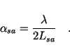
The angular resolution of a synthetic aperture of the length $L_{sa}$ is again given by the diffraction limit, and is two times higher as the one of a real aperture of the same length:

$\begin{displaymath}\alpha_{sa} = \frac{\lambda}{2 L_{sa}} \quad.\end{displaymath}$

(5)

The factor of `two' is the result of the synthetic aperture formation. The phase differences between elements of the synthetic aperture result from a two-way path difference and are, therefore, two times larger than in the case of a real antenna.

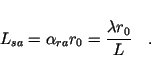
The maximum length for the synthetic aperture is the length of the flight path from which a scatterer is illuminated. This is equal to the size of the antenna footprint on the ground at the distance , where the scatterer is located at:

$\begin{displaymath}L_{sa} = \alpha_{ra} r_0 = \frac{\lambda r_0}{L} \quad.\end{displaymath}$

(6)

If the full synthetic aperture is formed, the azimuthal spatial resolution at the distance results as

$\begin{displaymath}\delta_{az} = \alpha_{sa} r_0 = \frac{L}{2} \quad.\end{displaymath}$

(7)

Interestingly, the achieved resolution is now completely independent of the range distance and is determined only by the size of the real antenna. This is a result of the increasing length of the synthetic aperture for longer distances to the object. In contrast to a SLAR, a shorter antenna now produces higher resolution because of its wider angular radiation characteristics. For higher flight heights, there still exists the problem of small backscattering power. Therefore, a sufficient long antenna is necessary for adequate focusing of the power. Due several technical limitations (available power, data-rate) a spaceborne SAR typically has lower resolution (approximately 5m) than an airborne SAR (up to 30cm). However, with SAR systems, high resolution radar imaging becomes possible even in the case of very long range distances.

Interpretation of SAR images

It is obvious that radar images look very different then optical remote sensing images. Because of the use of of different parts of the electromagnetic spectra, the information content is not comparable. Additionally, due to the different imaging geometries as well as the use of a coherent sensor system in the case of SAR, further differences are introduced. For a correct interpretation of SAR images therefore a detailed understanding of the characteristica of SAR images is necessary.

First of all, due to the coherent data recording, SAR images have complex pixel values (amplitude and phase), in contrast to optical images where only the image amplitude can be recorded. To achieve a SAR image, usually only the amplitude is used for the image brightness, as the images phase has a random distribution. Nevertheless, the image phase becomes important in SAR interferometry and polarimetry.

Looking at a distributed scatterer, i.e. an image pixel where many differnet individual scatterers are located, each of them has a contribution to the total backscattering. Due to the coherent radar wave, all individually backscattered wave interfere when forming to total signal. As depicted in Fig. 2.2, the result is the coherent vector sum of all contributions, which has a random phase, and a amplitude which is distributed about the true backscattering amplitude of the individual scatterers.

A characteristic of SAR images is therefore the so-called "speckle", which denotes the distribution of the measured amplitude around an average value, even over homogeneous areas. SAR images appear therefore not very "smooth", as it is well known for optical images. However, this is not a result of low resolution, but a direct result of the coherent imaging process. Examples for distributed targets are nearly all types of natural surfaces, like bare soil, meadows or forests.

4cm

$\includegraphics [scale=0.5]{vektoren.epsi}$

Figure 2.2: Coherent vector sum of individual scattering contributions inside one resolution element.

As point targets, scatterers are denoted, which have only one dominant scatterer signal in each resolution cell. This is the case for bigger metallic objects, other man-made targets like buildings, or radar-reflectors which have a stong reflection due to their geometry. In this case the measured amplitude and phase are a direct result of the reflectivity and phase shifts during the backscattering process. On such targets, the true image resolution can be estimated.

$\includegraphics [width=12cm,height=4cm]{layover.eps}$

Figure 2.3: Layover and shadow areas caused by terrain slope.

$\includegraphics [scale=0.5]{sarbsp.eps}$

Figure 2.4: Beispiel f"ur ein SAR-Bild, Gebiet: Sizilien, Sensor: ERS-1, C-Band

Further differences to optical images result from the different imaging geometry. With radar systems, time delays are measured, i.e. points in the same distance to the antenna are imaged at the same position in the imaged. This becomes a problem, if the examined area has strong topography. In Fig. 2.3, the interaction of a plane wavefront with a mountain is show. It can be observed, that the signal arrives at the same time at point 1 and 2. The whole area between 1 and 2 is therefore imaged at approximately the same position in the image, and cannot be resolved. Always if the surface slope exceeds the look-angle of the radar, the effect called 'layover' occurs. But also if the surface slope is smaller, the mountains seem to tilt towards the sensor, because the time delay from the top is reduced due to the larger topographic height.

On the backside of the mountains it can happen, that the radar signal is shadowed by the topography. In an optical image, which imaging technique is based on the measurment of angles, point 2 and 3 would appear at the same image position. In a radar image, where time delays are measured, between the response from point 2 and point 3, no echo is received. This causes an area in the image whithout backscattering, called 'shadow'. It contains only system noise and appears mostly black.

In order to give an impression, in Fig. 2.4 an ERS-a SAR image of a mountainous area in Sicily/Italy is shown. The geometric disturbances due to the topography as well as the speckle can easily be observed. Shadowing is not occuring here. ERS-1 has a very steep look-angle of $\vartheta=23^\circ$ and the effect occurs only for surface slopes greater than 90 $^\circ$ - $\vartheta$ .

Next: Processing of SAR-data Up: processing Previous: Short overview on SAR
Main level: Epsilon Nought - Radar Remote Sensing

Andreas Reigber
2001-05-24