


Next: Interpretation of Scattering Mechanisms
Up: Target Decomposition
Previous: The Vorticity Concept
Contents
In the previous section we discussed
deterministic scatterers which are described completely by a single
constant scattering matrix [S] or scattering vector  .
For remote sensing applications the assumption of pure deterministic
scatterers is not always valid, since, the resolution cell is usually bigger than the wavelength, e.g., natural
terrain surfaces contain many spatially distributed
scattering centers, the
measured [S]-matrix for a given resolution cell consists of the coherent
integration of all scattering contributions related to the particular
resolution cell. To deal with statistical scattering effects and the
analysis of extended scatterers, the concept of power reflection matrices is
traditionally preferred.
The classical and first decomposition related to this class of matrices
was presented by Huynen [2] in terms of an average single target component
matrix and a distributed residue component matrix. However, in
recent years, approaches based on the coherence and covariance matrices
have been preferred because of their more compact form. The coherence and covariance matrices as well as the Müller/Kennaugh matrices belong to this type of power reflection matrices. They hold identical information only in a different representation. Therefore, these representations can be mutually transfered from one into the other without loss of information. Depending on the desired information the one or the other representation may yield some advantages. However, for radar remote sensing applications coherence matrix representation is usually preferred, due to the fact, that the analysis of this matrix by means of the Cloude decomposition theorem is straight forward. Therefore, we shall be focus on the coherence matrix and the Cloude decomposition theorem in the following.
.
For remote sensing applications the assumption of pure deterministic
scatterers is not always valid, since, the resolution cell is usually bigger than the wavelength, e.g., natural
terrain surfaces contain many spatially distributed
scattering centers, the
measured [S]-matrix for a given resolution cell consists of the coherent
integration of all scattering contributions related to the particular
resolution cell. To deal with statistical scattering effects and the
analysis of extended scatterers, the concept of power reflection matrices is
traditionally preferred.
The classical and first decomposition related to this class of matrices
was presented by Huynen [2] in terms of an average single target component
matrix and a distributed residue component matrix. However, in
recent years, approaches based on the coherence and covariance matrices
have been preferred because of their more compact form. The coherence and covariance matrices as well as the Müller/Kennaugh matrices belong to this type of power reflection matrices. They hold identical information only in a different representation. Therefore, these representations can be mutually transfered from one into the other without loss of information. Depending on the desired information the one or the other representation may yield some advantages. However, for radar remote sensing applications coherence matrix representation is usually preferred, due to the fact, that the analysis of this matrix by means of the Cloude decomposition theorem is straight forward. Therefore, we shall be focus on the coherence matrix and the Cloude decomposition theorem in the following.
The Cloude decomposition theorem is capable of covering a whole range of scattering mechanisms is based on the eigenvector
analysis of the coherence matrix [T] and was first presented by Cloude [Cloude85], [Cloude92].
This approach yields the important advantage, that it is automatically basis invariant due to the
invariance of the eigenvalue problem under unitary transformations.
Due to the fact that the coherence matrix [T] is a hermitian, positive, semidefinite matrix,
it can always be diagonalized, using unitary similarity transformations [Cloude97]. That is, the coherency
matrix may be given as
![$\displaystyle \left<[T]\right>=[U_3][\Lambda][U_3]^{\dagger}=[U_3]
\left[ \begi...
... & 0 & \lambda_3
\end{array} \right]
[U_3]^{\dagger} \qquad where \qquad \qquad$](img310.gif) |
|
|
|
![$\displaystyle \left[U_3 \right] = \left[ \begin{array}{ccc}
\cos(\alpha_1) &
\c...
..._2)e^{i\gamma_2} &
\sin(\alpha_3)\sin(\beta_3)e^{i\gamma_3}
\end{array} \right]$](img311.gif) |
|
|
(4.17) |
where ![$ [\Lambda]$](img312.gif) is the diagonal eigenvalue matrix of [T],
is the diagonal eigenvalue matrix of [T],
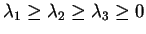 are the real eigenvalues and
![$ [U_3]$](img314.gif) is a unitary matrix whose columns correspond to the orthonormal eigenvectors
is a unitary matrix whose columns correspond to the orthonormal eigenvectors
 of [T].
Thus the coherence matrix [T] can be decomposed into a sum of 3
coherence matrices ![$ [T_n]$](img316.gif) , each weighted by its corresponding eigenvector.
, each weighted by its corresponding eigenvector.
![$\displaystyle [T] = \sum_{n=1}^3 \lambda_n [T_n] = \lambda_1 (\vec{e}_1 \cdot \...
...c{e}_2 \cdot \vec{e}_2^\dagger) + \lambda_3 (\vec{e}_3 \cdot \vec{e}_3^\dagger)$](img317.gif) |
(4.18) |
Each matrix is a unitary scattering matrix representing a deterministic scattering contribution.
The amount of the contributions is given by the eigenvalues  while the type of scattering is related to the eigenvectors.
Two important physical features arising from this decomposition where introduced by Cloude
and Pottier [Cloude97]
The first one is the polarimetric scattering entropy H which is a global measure of the
distribution of the components
of the scattering process and is defined as
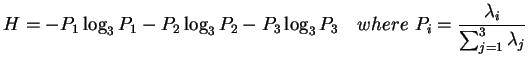 |
(4.19) |
where  may be interpreted as the relative intensity of
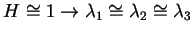
a scattering process 'i'. Due to this definition H is restricted to the interval
0
may be interpreted as the relative intensity of
a scattering process 'i'. Due to this definition H is restricted to the interval
0  H 1, where H = 0 indicates that [T] has only one nonzero eigenvalue and
represents one deterministic scattering process,
while H = 1 means that all are equal.
H 1, where H = 0 indicates that [T] has only one nonzero eigenvalue and
represents one deterministic scattering process,
while H = 1 means that all are equal.
Since the entropy is mainly an indicator for the relationship between  and the
two other eigenvalues
and the
two other eigenvalues  ,
,  , no direct information about the relation between the latter
can be extracted from the entropy. The second feature, introduced by Pottier [Pottier98a],
the polarimetric anisotropy A,
, no direct information about the relation between the latter
can be extracted from the entropy. The second feature, introduced by Pottier [Pottier98a],
the polarimetric anisotropy A,
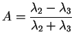 |
(4.20) |
closes this gap.
For a high entropy the anisotropy yields no additional information since in that case
the eigenvalues are nearly equal (
 ).
For very low entropy we find, that the minor eigenvalues and are close to zero.
For low or medium entropy (
).
For very low entropy we find, that the minor eigenvalues and are close to zero.
For low or medium entropy (
 ), however, the entropy yields no
information about the relation between the two minor eigenvalues
), however, the entropy yields no
information about the relation between the two minor eigenvalues
 .
In that case the anisotropy contains additional information. A medium entropy means that more than one scattering mechanism
contributes to the signal, but not if one or two additional scattering mechanisms are present.
A high anisotropy states that only the second scattering mechanism is important, while a low anisotropy
yields that also the third scattering mechanism plays a role.
Possible applications of these features for classification purposes are given in [Pottier98b] and shall
be discussed in the following chapter.
.
In that case the anisotropy contains additional information. A medium entropy means that more than one scattering mechanism
contributes to the signal, but not if one or two additional scattering mechanisms are present.
A high anisotropy states that only the second scattering mechanism is important, while a low anisotropy
yields that also the third scattering mechanism plays a role.
Possible applications of these features for classification purposes are given in [Pottier98b] and shall
be discussed in the following chapter.
Next: Interpretation of Scattering Mechanisms
Up: Target Decomposition
Previous: The Vorticity Concept
Contents